(or “Why Decisions are Like Lava Pits”)
In daily life, we are seldom given “either-or” choices.

Okay, it still happens sometimes…
Often, when we make decisions, we have a multitude of choices to contend with. Sifting through these possibilities can be tricky, since we only have a limited set of observations.
In statistics, we call this challenge “Multiple Testing”, and it can quickly lead to faulty decision-making.
Why Multiple Testing is Dangerous
When we test a hypothesis, we are making a yes-no decision as to whether our data indicates a finding.
Each time you use data to take an inductive “leap”, there is some risk that you will be mistaken. This is what we mean when we talk about being 95% confident.
To illustrate this danger, let’s play a simple children’s game…
The Floor is Lava!
The floor has suddenly grown much hotter. In fact, it is now completely molten.
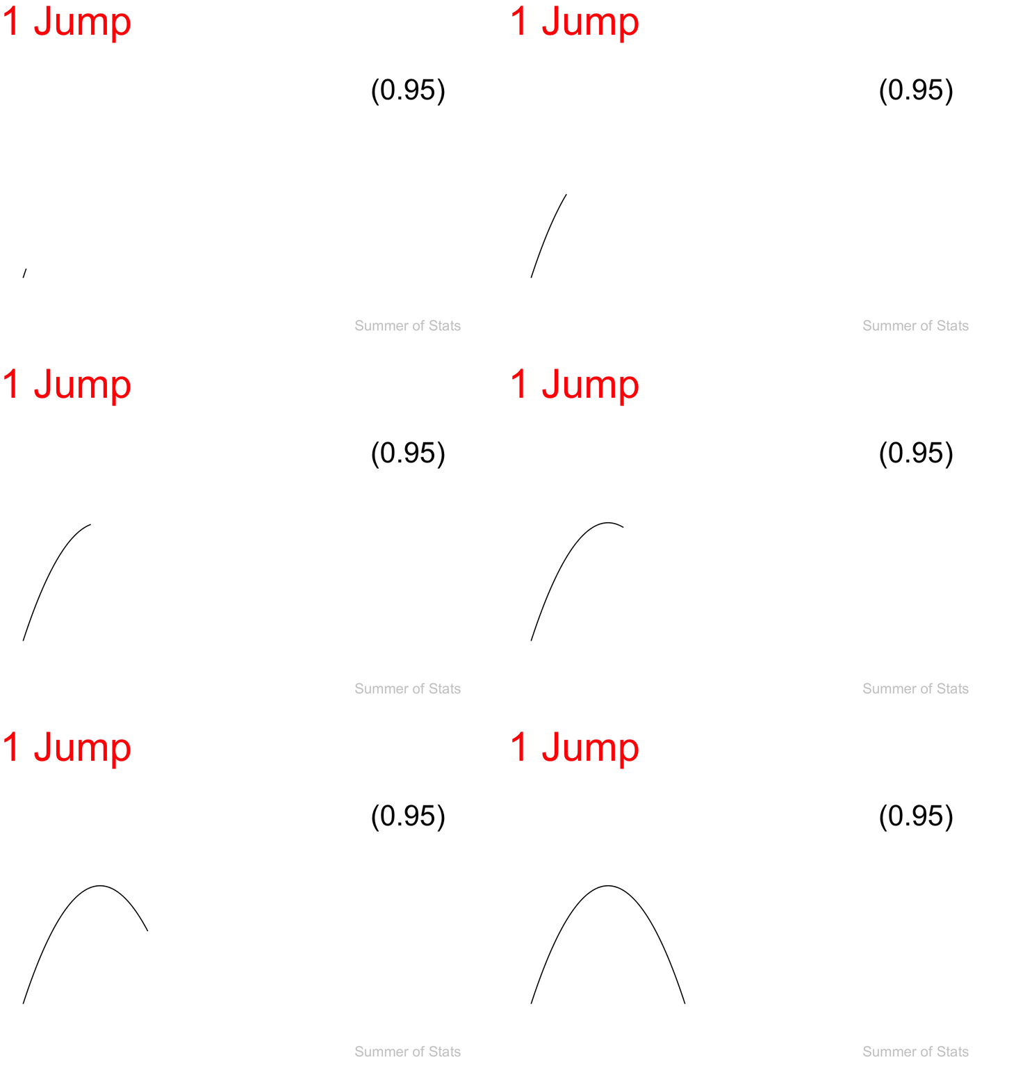
To escape, you must leap across the lava to a nearby platform. You’re reasonably agile, so you’ll most likely make it. Let’s peg your odds at 95%.
If you don’t make it, well….let’s not dwell on that.

Probability of Survival: 95%
You made it! But now, you have to make another jump to progress.
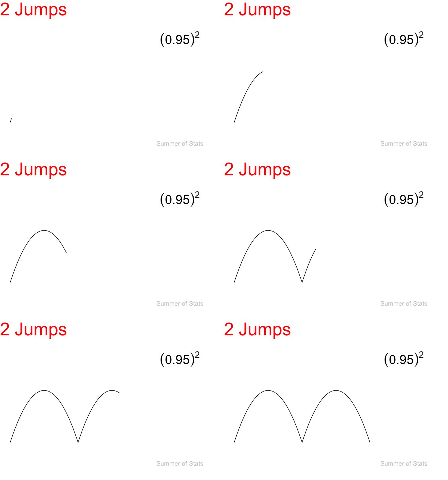
This jump (conveniently) ALSO has a 95% success rate, so you have to be a bit luckier to complete both jumps successfully:

Probability of Survival: 90.25%
So far, so good.
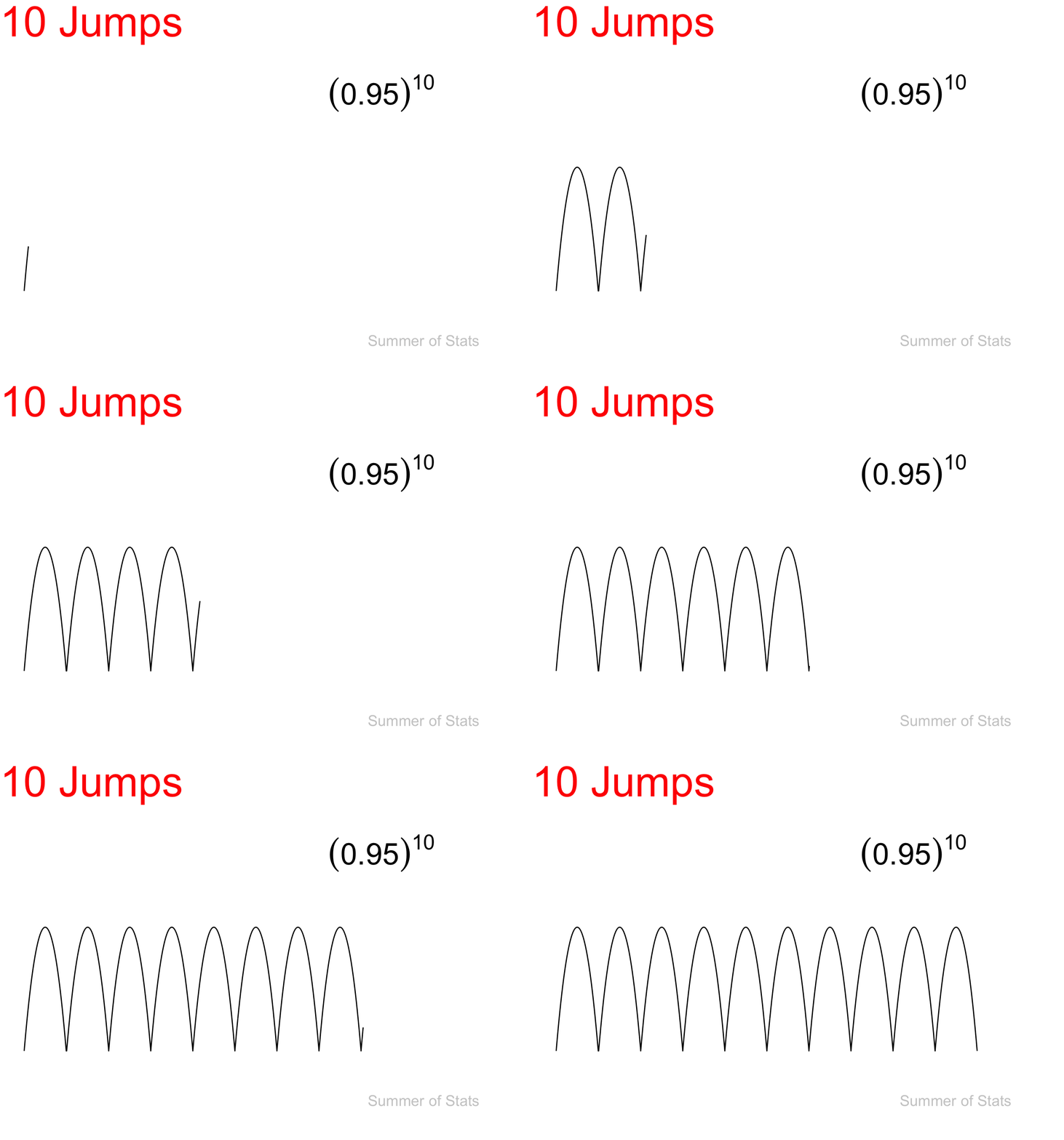
And now, just 8 MORE jumps, and you’ve made it to freedom!

Probability of Survival: 59.87%
Congratulations, you’ve (probably) survived the world’s most intense game of Floor is Lava!
The Takeaway
As you can see, the odds of succeeding EVERY single time shrink quickly, even when each individual step has a pretty high probability.
Leap once, and things aren’t so bad. But, once you start testing dozens (or even hundreds) of hypotheses with the same data, you’re very likely to decide wrong.
Multiple Testing in Daily Life
One practical lesson that you can take away is:
Beware of simply “following the data”
Often, analysts are given data, with the cryptic instruction to “Find what the data tells us”.
Unfortunately, extremely open questions like this one are not well suited to statistical inference, as we’ll see below.
A Random Dataset
Let’s generate a dataset to do data mining against. Since people love Big Data, we’ll make it have 100,000 observations.
The catch is that our data is completely random - the outcome is a randomly generated number, and our “treatments” are a randomly generated letter of the alphabet.
Let’s run a regression on this data to see what happens:
##
## Call:
## lm(formula = Outcome ~ ., data = random_data)
##
## Residuals:
##      Min       1Q   Median       3Q      Max
## -30.4688  -4.7282   0.0342   4.7068  29.0064
##
## Coefficients:
##              Estimate Std. Error t value Pr(>|t|)
## (Intercept) -0.179191   0.112066  -1.599   0.1098
## Letter_B     0.120609   0.159467   0.756   0.4495
## Letter_C     0.162456   0.159152   1.021   0.3074
## Letter_D     0.174951   0.159090   1.100   0.2715
## Letter_E     0.178524   0.159288   1.121   0.2624
## Letter_F     0.153234   0.159509   0.961   0.3367
## Letter_G     0.290290   0.159236   1.823   0.0683 .
## Letter_H     0.198189   0.159701   1.241   0.2146
## Letter_I     0.316057   0.158770   1.991   0.0465 *
## Letter_J     0.262196   0.158780   1.651   0.0987 .
## Letter_K     0.172178   0.158945   1.083   0.2787
## Letter_L     0.128438   0.159351   0.806   0.4202
## Letter_M    -0.017988   0.158163  -0.114   0.9095
## Letter_N     0.057193   0.158893   0.360   0.7189
## Letter_O     0.006871   0.158790   0.043   0.9655
## Letter_P    -0.060487   0.159509  -0.379   0.7045
## Letter_Q     0.281731   0.159754   1.764   0.0778 .
## Letter_R     0.259364   0.158770   1.634   0.1023
## Letter_S     0.074578   0.158495   0.471   0.6380
## Letter_T     0.131117   0.159851   0.820   0.4121
## Letter_U     0.320497   0.159626   2.008   0.0447 *
## Letter_V     0.055689   0.159840   0.348   0.7275
## Letter_W     0.203604   0.158657   1.283   0.1994
## Letter_X     0.192837   0.160449   1.202   0.2294
## Letter_Y     0.236105   0.160219   1.474   0.1406
## Letter_Z     0.342401   0.158394   2.162   0.0306 *
## ---
## Signif. codes:  0 '***' 0.001 '**' 0.01 '*' 0.05 '.' 0.1 ' ' 1
##
## Residual standard error: 7.012 on 99974 degrees of freedom
## Multiple R-squared:  0.000242,	Adjusted R-squared:  -7.988e-06
## F-statistic: 0.968 on 25 and 99974 DF,  p-value: 0.5078
A Significant Finding?
We see that running a regression against this random dataset generated 3 “significant” findings (“I”, “U”, and “Z”) despite these variables having no actual connection to our outcome of interest.
Note that this result is not surprising - if we use the standard 95% confidence, then we accept a 5% risk that our finding is due to random chance.
Now do this 26 times:
$$ 0.05 * 26 = 1.3 $$
So, if we test 26 variables simultaneously at 95% confidence, we should expect around 1.3 false findings in our results!
A Significant Problem
As datasets get bigger and better, the temptation is to search for ANY possible finding within the dataset. But our example above should give you pause about putting too much confidence on these findings when many, many variables are involved.
Summing Up
Every decision we make is a leap of faith. But not all leaps of faith are created equal.
To avoid Multiple Testing you have to be picky: Clearly specify what you are looking for up-front. By running fewer tests, you make it less likely you see a false positive.
Or, if you MUST explore many possibilities, consider doing a follow-up study to see whether the pattern you saw in the initial data holds up in the new data you collect.
While any good fact-finder should keep an open mind, when you start testing every possibility, you’re likely to make faulty decisions.
Up Next: Missing Data
Next week, we’ll discuss how missing data can impact your results.
Find out why the data you DIDN’T collect is often the most important part of your analysis.
===========================
R code used to generate plots:
- Lava Hopping
library(data.table)
library(ggplot2)
library(gganimate)

arc <- data.table(
    x = seq(-50, 50, by = 1),
    time = seq(0, 100, by = 1)
)

arc[,y:= -0.01 * x^2]

leap_1 <- ggplot(arc, aes(x=x, y=y)) +
    geom_line() +
    coord_cartesian(ylim=c(-40, 20), xlim=c(-50, 250)) +
    theme_void() +
    theme(plot.title=element_text(family='', face='bold', size=40, color="red")) +
    ggtitle("1 Jump") +
    annotate("text", x = 200, y = -35, label = "Summer of Stats", col="grey80", size = 5) +
    transition_reveal(time, keep_last = TRUE)

animate(leap_1, duration = 2, end_pause = 50)

## Duplicate data for 2nd jump
arc_2 <-rbind(arc,arc)
arc_2[100:201, x:=x+100]
arc_2[100:201, time:=time+100]


leap_2 <- ggplot(arc_2, aes(x=x, y=y)) +
    geom_line() +
    coord_cartesian(ylim=c(-40, 20), xlim=c(-50, 250)) +
    theme_void() +
    theme(plot.title=element_text(family='', face='bold', size=40, , color="red")) +
    ggtitle("2 Jumps") +
    annotate("text", x = 200, y = -35, label = "Summer of Stats", col="grey80", size = 5) +
    transition_reveal(time, keep_last = TRUE)

animate(leap_2, duration = 3, end_pause = 50)

## Duplicate data for 10 jumps
arc_10 <-rbind(arc,arc,arc,arc,arc,arc,arc,arc,arc,arc,arc)
arc_10[,indx:=.I]
arc_10[,f_indx := floor((indx - 2)/ 100) * 100 ]
arc_10[102:1111, x:=x+f_indx+1]
arc_10[102:1111, time:=time+f_indx+1]
arc_10 <- arc_10[1:1000]


leap_10 <- ggplot(arc_10, aes(x=x, y=y)) +
    geom_line() +
    coord_cartesian(ylim=c(-40, 20), xlim=c(-50, 1100)) +
    theme_void() +
    theme(plot.title=element_text(family='', face='bold', size=40, , color="red")) +
    ggtitle("10 Jumps") +
        annotate("text", x = 900, y = -35, label = "Summer of Stats", col="grey80", size = 5) +
    transition_reveal(time, keep_last = TRUE)

animate(leap_10, duration = 9, end_pause = 50)
- Random Regression
set.seed(073025)

random_data <- data.table("Outcome" = rnorm(100000,0,7),
                          "Letter_" = LETTERS[runif(100000,1,27)])

test_lm <- lm(Outcome ~ ., random_data)
summary(test_lm)