(or “Why Plaid Will Never Go Out of Style”)
Knowing when to change your mind about something is one of the toughest things we have to do.

“Maaaaybe it’s time to update my wardrobe…”
Over time, we may see evidence pop up that contradicts our opinion. But, how do we know when there’s enough evidence for us to change our minds?
One way we can approach this problem analytically is with Bayesian statistics.
What is Bayesian Statistics?
Bayesian statistics is a very different approach to statistics.
- So far, we’ve modeled our analysis based on long-term expectations and some simplifying assumptions (usually based on the normal distribution).
- With Bayesian statistics, we make an initial statement of how we believe things work, and then update that belief based on the data we collect.
Let’s show this process in action!
Our Initial Belief (Prior): “People Like Plaid, Right?”
Let’s say that you have an old plaid suit that you love. You are wondering if you should keep it, or buy a newer suit.
Based on years of experience, you believe that plaid suits are IN.
Okay, the reality is, you’ve had a few people comment on that suit, and MOST of them seemed complimentary (note: you don’t have a good ear for sarcasm…).
As a result, you believe that ~70% of people like the suit. To model this, we create our prior distribution, and center it at 70%:
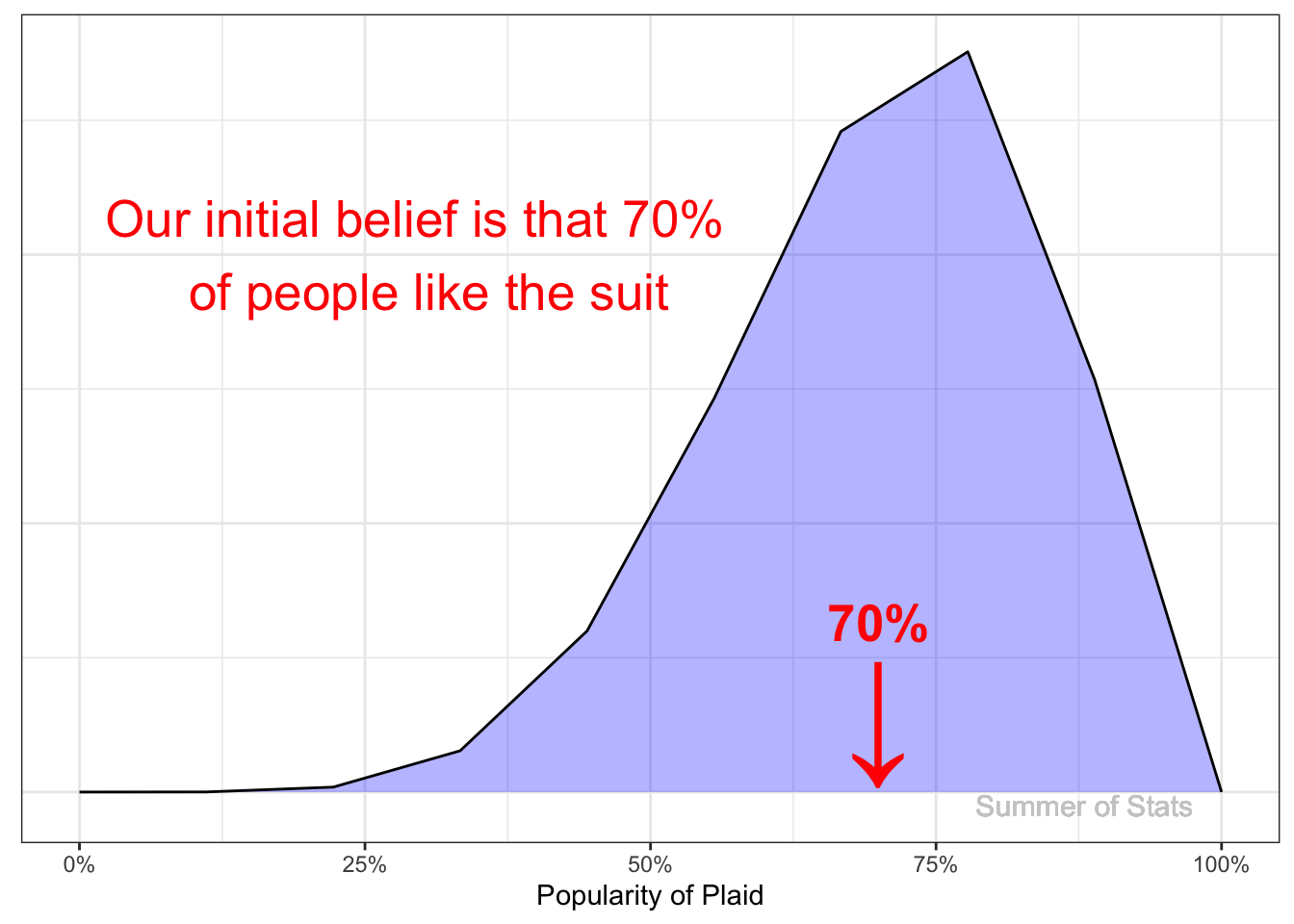
However, we’re not super-sure about our initial evidence, so we make our distribution a bit wider. We call this a “weak” prior.
Translating our prior into plain English, we could say:
“We believe that a majority people (~50%-100%) probably like plaid, but we don’t know much more than that.”
The Data: “Nope”
To test our theory, we survey 100 different people* about whether plaid is a good look. Only 7 out of 100 people agreed.
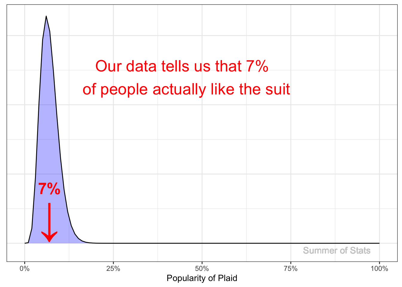
*Note: We don’t even have to be the ones to collect this data. We could have just as easily read this in a magazine…what matters is that we believe in the results.
This finding is clearly at odds with our initial belief - so how do we reconcile these conflicting findings?
We can use Bayes’ theorem to decide what to do next!
The Result (Posterior): “Maybe I Should Get a New Suit…”
Based on the new data, we update our beliefs.
Mathematically, this is done by combining the beta distributions of our prior + likelihood (aka. our collected data): $$ Prior + Likelihood = Posterior $$
$$ Beta(7,10) + Beta(7,100) = \bf{Beta(14,110)}$$
Our new belief is centered around 13% of people liking plaid, rather than our initial belief of 70% :
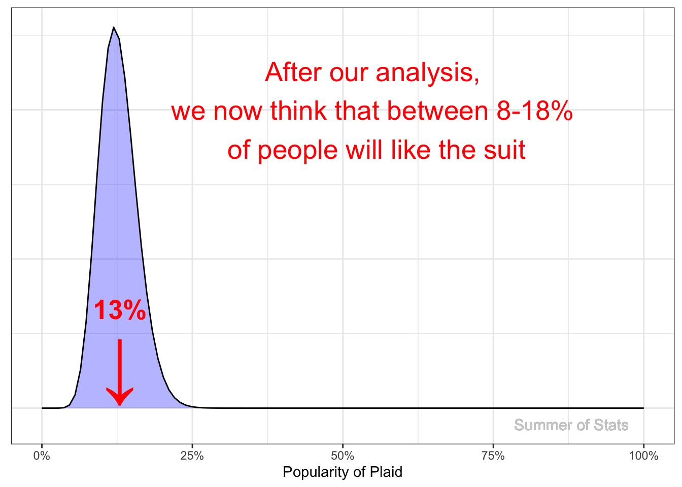
In the end, we still hold out some hope (based on our prior belief) that the survey overestimated people’s hatred for plaid, but have largely accepted the evidence.
From this analysis, we can clearly see that it’s time to invest in a new suit.
It’s All About Beliefs
But what if we were REALLY sure that we looked good in plaid?
Bayesian statistics allows for this too. By choosing a “stronger” prior, we can express “stronger” belief in our prior knowledge. At a certain point, even the strong signal we get from our data may not sway our opinion.
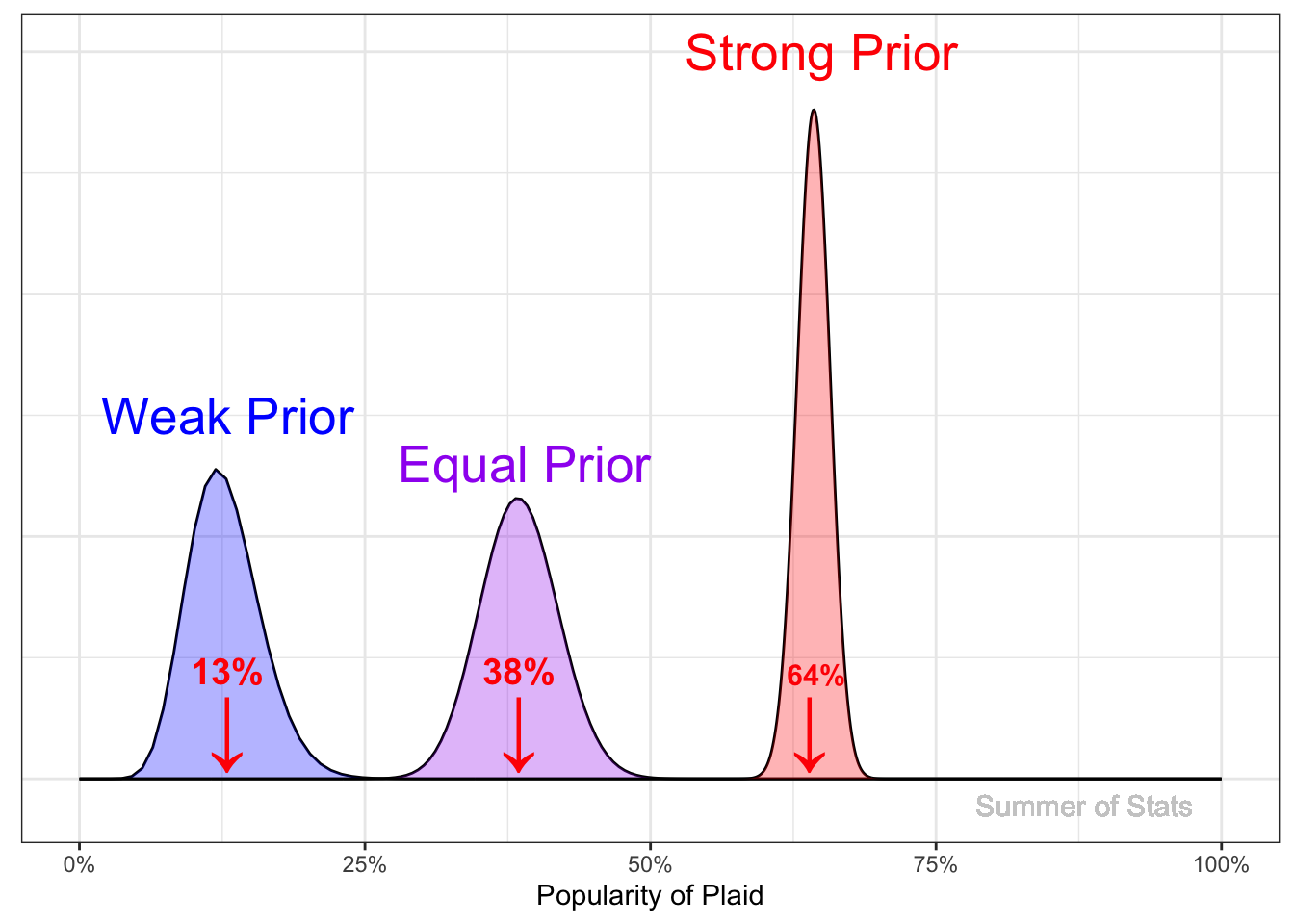
This example illustrates an important feature of Bayesian inference - the strength of your prior belief influences your outcome.
Bayesian Statistics in Daily Life
One practical lesson of Bayesian statistics that you can take away is:
There’s no such thing as a truly “objective” analysis.
Bayesian statistics often gets flak for letting subjective beliefs affect the outcome. However, traditional statistical analysis can be just as subjective.
Let’s briefly illustrate how easy it is to unintentionally bias an analysis, using an all-too-common scenario…
“Can You Find Me Some Data?”
Many analysts have been given an assignment similar to the one below:
“We are going to propose adding a Repair Center to stores - can you find some data about the effect on profitability?”
Simple enough. We crunch some numbers, make a basic financial projection, and find that adding this to stores increases profitability. Sounds good, right?
Wrong.
What we DIDN’T find was also important. In the end, the program increased workload at the store considerably (repairs are often very time-consuming). This added workload led to worse customer service, costly mistakes, and increased employee turnover.
While the initiative successfully generated SOME revenue, it clearly harmed profitability overall.
Not a good result…
What Went Wrong?
Our analysis was off because the request focused on only one aspect of the proposal (financial). This clear bias made it less likely we’d find other reasons to NOT move forward with the initial proposal.

“I propose we burn all of our money to increase profitability - it’ll decrease our cash-handling costs!”
In this case, an innocuous-sounding decision early on about what to focus on had a huge effect on our outcome - a Bayesian might say that’s not much different than having a strong prior!
Summing Up
By using data to update beliefs, Bayesian statistics provide a flexible approach to tackling difficult problems.
This technique pops up in many places: filtering spam emails, diagnosing diseases, and even locating unexploded nuclear weapons.
With Bayesian statistics, it is critical to have reasonable beliefs. As we saw with our plaid suit fan, if our prior beliefs are too strong, no amount of evidence will be able to sway our opinion. And sometimes a change of mind can do us a lot of good…
Next week, we’ll explore the science of how to collect our data, using Design of Experiments.
===========================
R code used to generate plots:
library(data.table)
library(ggplot2)
library(scales)
set.seed(060124)


### function to create a beta dist, for plotting in ggplot
create_beta_dist <- function(var_Successes, var_N) {

  beta_dist <-cbind(seq(0, 1, length=var_N),
          dbeta(seq(0, 1, length=var_N), var_Successes, var_N - var_Successes)) |> as.data.table()

}

### function to create a uniform base plot, to be annotated for each
plot_beta_dist <- function(beta_dist) {

  ggplot(beta_dist, aes(x=V1, y=V2)) +
  geom_area(position = "identity", fill="blue", alpha = 0.3) +
  geom_line() +
  theme_bw() +
  xlab("Popularity of Plaid") +
  theme(axis.text.y=element_blank(),
        axis.ticks.y=element_blank(),
        axis.title.y=element_blank()) +
  scale_x_continuous(label=label_percent()) +
    geom_text(data = beta_dist, aes(x = .88, y = (-.5)* beta_dist[,.N]/100, label = "Summer of Stats"), col="grey80", size = 4)

}

### Plot beta dist for prior
create_beta_dist(7, 10) |>
  plot_beta_dist() +
  annotate("text", x = .3, y = 2, label = "Our initial belief is that 70% \n of people like the suit", col = "red", size = 7) +
  annotate("text", x = .70 , y = .71, label = 'atop(bold("70%"))', col = "red", size = 7, parse = TRUE) +
  annotate("text", x = .70 , y = 0, label = 'atop(bold("↓"))', col = "red", size = 20, parse = TRUE)

### Plot beta dist for data
create_beta_dist(7, 100) |>
  plot_beta_dist() +
    annotate("text", x = .45, y = 12, label = "Our data tells us that 7% \n of people actually like the suit", col = "red", size = 7) +
  annotate("text", x = .07 , y = 3.5, label = 'atop(bold("7%"))', col = "red", size = 7, parse = TRUE) +
  annotate("text", x = .07 , y = 0, label = 'atop(bold("↓"))', col = "red", size = 20, parse = TRUE)

### Plot beta dist for posterior
create_beta_dist(14, 110) |>
  plot_beta_dist() +
    annotate("text", x = .55, y = 10, label = "We now think that between 8-18% \n of people will like the suit", col = "red", size = 7) +
    annotate("text", x = .13 , y = 3, label = 'atop(bold("13%"))', col = "red", size = 7, parse = TRUE) +
  annotate("text", x = .13 , y = 0, label = 'atop(bold("↓"))', col = "red", size = 20, parse = TRUE)


### Let's consider alternate priors:
weak_prior <- create_beta_dist(14,110)  # Prior = beta(7,10)
equal_prior <- create_beta_dist(77, 200) # Prior = beta(70, 100)
strong_prior <- create_beta_dist(707, 1100) # Prior = beta(700,)


  ggplot(weak_prior, aes(x=V1, y=V2)) +
  # Weak Prior
  geom_line(data=weak_prior, aes(x=V1, y=V2)) +
  geom_area(position = "identity", fill="blue", alpha = 0.3) +
  annotate("text", x = .13, y = 15, label = "Weak Prior", col = "blue", size = 7) +
  # Equal Weight
  geom_line(data=equal_prior, aes(x=V1, y=V2)) +
  geom_area(data=equal_prior, aes(x=V1, y=V2), position = "identity", fill="purple", alpha = 0.3) +
  annotate("text", x = .39, y = 13, label = "Equal Prior", col = "purple", size = 7) +
  # Strong Prior
  geom_line(data=strong_prior, aes(x=V1, y=V2)) +
  geom_area(data=strong_prior, aes(x=V1, y=V2), position = "identity", fill="red", alpha = 0.3) +
  annotate("text", x = .65, y = 30, label = "Strong Prior", col = "red", size = 7) +
  theme_bw() +
  xlab("Popularity of Plaid") +
  theme(axis.text.y=element_blank(),
        axis.ticks.y=element_blank(),
        axis.title.y=element_blank()) +
  scale_x_continuous(label=scales::label_percent()) +
  geom_text(data = weak_prior, aes(x = .88, y = -.1*strong_prior[,.N]/100, label = "Summer of Stats"), col="grey80", size = 4)  +
    annotate("text", x = .13 , y = 3.3, label = 'atop(bold("13%"))', col = "red", size = 5, parse = TRUE) +
  annotate("text", x = .13 , y = 0, label = 'atop(bold("↓"))', col = "red", size = 12, parse = TRUE) +
    annotate("text", x = .385 , y = 3.3, label = 'atop(bold("38%"))', col = "red", size = 5, parse = TRUE) +
  annotate("text", x = .385 , y = 0, label = 'atop(bold("↓"))', col = "red", size = 12, parse = TRUE) +
    annotate("text", x = .645 , y = 3.3, label = 'atop(bold("64%"))', col = "red", size = 4, parse = TRUE) +
  annotate("text", x = .64 , y = 0, label = 'atop(bold("↓"))', col = "red", size = 12, parse = TRUE)