(or “Why It Pays to be a Communications Major”)
Nearly every topic we’ve covered so far has relied on a BIG assumption: that our data looks somewhat like this:
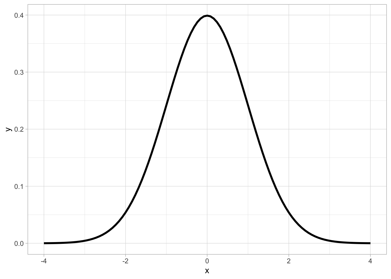
But what if your data doesn’t fit a distribution nicely? What if your data is very skewed, irregular, or has big outliers?
Time to bring in nonparametric statistics!
What is a Nonparametric Statistic?
In short, a nonparametric statistic is a more robust option for analyzing data. It achieves this by essentially ignoring the actual values in your data, and converting each to a rank.
This approach shines when we have highly skewed data and/or outliers, since it produces results that aren’t swayed by extreme or unusual values.
As we’ll see below, this property can be very useful.
Mean vs. Median
A nonparametric statistic that all of us are familiar with is the median.
Its parametric cousin (the mean) is more widely used, but the median can provide a more accurate picture when our data is skewed, since is not influenced by extreme outliers.
Let’s see this in action!
Notice how much the mean “jumps” in response to an outlier. Meanwhile, the median doesn’t even flinch:
In this case, we see how the mean overestimates where the “center” of our data is.
Statistics for Larger Sample Sizes
Luckily, when we have more data points, the effects of an extreme outlier can be mitigated without having to use a nonparametric approach.
Here, we see that after just 30 observations, the outlier’s effect on the mean is very small:
As a result, nonparametric statistics are most valuable when dealing with small sample sizes and large outliers.
Other Uses of Nonparametric Statistics
There are corresponding nonparametric approaches to nearly everything we’ve discussed so far:
- With highly skewed data, traditional hypothesis tests can become problematic.
- Outliers are a clear problem for linear regression, and can easily ruin your model.
- Calculating confidence intervals from irregular data is also sticky.
Further reading
Because there is far too much to cover on each of these to fit into a single post, here are some interesting reads on each:
Hypothesis Testing: This short lesson has a great example of how using a nonparametric hypothesis test can prevent a biased result.
Regression: Robust regression methods exist, such as the ones outlined in this quick guide.
Confidence Intervals: Check out this eye-opening article on how to use bootstrap resampling to generate reasonable confidence intervals, even with skewed data.
Nonparametric Statistics in Daily Life
One practical lesson of nonparametric statistics that you can take away is:
Be wary of averages.
Everyone knows the old quote about “lies, damned lies, and statistics”. Well, 99% of those lies are told by averages.
Let’s pick one of these apart, using nonparametric statistics…
When Averages Lie
Back in undergrad, I learned about lying with statistics from a college proclaiming the “high average salary” of their communications majors.
However, inspecting further, there was something a bit fishy about their claims:
| Major | Average Starting Salary |
|---|---|
| Chemical Engineering | $66,000 |
| Communications | $65,000 |
| Computer Science | $55,000 |
| Nursing | $54,000 |
Seems a BIT high, doesn’t it?
If the college was being a bit more honest, they would’ve provided the MEDIAN salary, which unfortunately (for them) looked much less impressive.
| Major | MEDIAN Starting Salary |
|---|---|
| Math | $45,000 |
| Geology | $44,000 |
| Communications | $43,000 |
| Agriculture | $42,000 |
In reality, this specific college had an NBA star as an alumnus. That one person’s extreme salary pulled up the entire average for Communications majors, despite not even being employed within the area covered by his degree.
Saved by the Median
Using the median of this data set immediately resolves the issue. No matter if our Pro Athlete made $10 million or $10 trillion dollars, the median salary for his college program would remain unchanged.
With averages, we can easily boost the result by introducing a single outsized value. The only way to “boost” the median is by raising the salaries of a large cohort of recent graduates. And THAT kind of gaming I can live with…
Summing Up
Outliers can pop up in any dataset, and cause real problems for accurately summarizing and analyzing data.
As a more conservative option, nonparametric analyses will handle these situations more gracefully. As we saw with salary statistics, one exceptional data point can completely alter the story when we use traditional statistics.
However, there is no free lunch - nonparametric approaches also generally have less statistical power than approaches we’ve covered to date. So, unless there’s a compelling data issue driving you, you are generally safe to stick with the normal (parametric) approaches we’ve covered.
Next week, we will be discussing yet another approach to analyzing data: Bayesian statistics.
Instead of avoiding assumptions (like nonparametric statistics), Bayesian statistics will actually require us to make assumptions before we even look at the data. The result is a totally new way to look at problems.
===========================
R code used to generate plots:
library(data.table)
library(ggplot2)
library(gganimate)
set.seed(060124)

right_skew <- rnorm(5, 10, 10) |> append(200) |> append(rnorm(4, 10, 10)) |> as.data.table()
right_skew[,Indx := .I]
right_skew[,c_mean:=cumsum(V1)/Indx]
right_skew[,c_median := vapply(seq_along(V1), function(i) median(V1[1:i]), 1)]

small_n <- ggplot(right_skew, aes(x=Indx, y=V1)) +
  geom_line() +
  geom_point() +
  geom_text(aes(y=right_skew$c_mean + 4, x = 12, label = "--MEAN--"), col = "red") +
  geom_text(aes(y=right_skew$c_median + 4, x = 14, label = "--MEDIAN--"), col = "black") +
  xlab("x") +
  ylab("y") +
  geom_text(aes(x = 13,
                y = -5,
                label = "Summer of Stats"), col="grey80", size = 3) +
   transition_reveal(Indx, keep_last = TRUE)

animate(small_n, duration = 6, renderer = gifski_renderer(loop = T))

extra_obs <- rnorm(5, 10, 10) |> append(200) |> append(rnorm(24, 10, 10)) |> as.data.table()
extra_obs[,Indx := .I]
extra_obs[,c_mean:=cumsum(V1)/Indx]
extra_obs[,c_median := vapply(seq_along(V1), function(i) median(V1[1:i]), 1)]

large_n <- ggplot(extra_obs, aes(x=Indx, y=V1)) +
  geom_line() +
  geom_point() +
  geom_text(aes(y=extra_obs$c_mean + 4, x = 35, label = "--MEAN--"), col = "red") +
  geom_text(aes(y=extra_obs$c_median + 4, x = 41, label = "--MEDIAN--"), col = "black") +
  xlab("x") +
  ylab("y") +
  geom_text(aes(x = 38,
                y = -5,
                label = "Summer of Stats"), col="grey80", size = 3) +
   transition_reveal(Indx, keep_last = TRUE)

animate(large_n, duration = 12, renderer = gifski_renderer(loop = T))