(or “Are These Eggs Still Good?”)
When we collect data, we are usually doing it to help make a decision.
For example: Is our machine filling each milk bottle consistently?

As we saw last week, the more data we collect, the more confident we generally feel about what we observe. But, how do we KNOW when we have enough evidence to draw a solid conclusion?
To tackle this problem, we use a technique called hypothesis testing.
What is A Hypothesis Test?
Hypothesis testing is a process that allows us to test our assumptions about the world.
There’s some math involved, but the high-level steps are pretty simple:
- We explicity state how we think things work (the null hypothesis)
- We collect some data (our sample)
- We calculate whether our result is different enough to contradict our null hypothesis (the hypothesis test)
To introduce this idea, let’s start with a simple question:
Are Basketball Players Taller?
In an earlier post on sampling, we saw that our sample of basketball players tended to be taller than the average male.
But, is this difference significant enough to conclude that basketball players (as a group) are shorter/taller than normal? Let’s measure heights from 100 people in each group, and compare the confidence intervals:
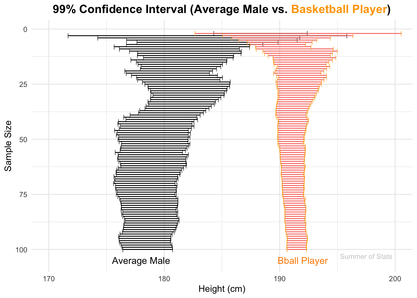
Initially, the height range of the 2 groups overlap, meaning that there is no strong evidence of a difference. But, as we add more observations we quickly see that the likely ranges for each group split off from each other.
By the time we’ve seen 100 people from each group, we are pretty sure the average heights of each group ARE different.
Testing Our Hypothesis
Let’s test our hypothesis formally, just to be sure. We will be using Welch’s t-test, since we have to estimate BOTH groups’ heights (average male and basketball player) with a sample of data.
To run the test in R, we just type:
t.test(sample1, sample2)
The Result
Our p-value is < 0.01, so we have strong evidence that there IS a difference between our groups.
##
## 	Welch Two Sample t-test
##
## data:  good_sample$V2 and bball_sample$V2
## t = -14.397, df = 128.59, p-value < 2.2e-16
## alternative hypothesis: true difference in means is not equal to 0
## 99 percent confidence interval:
##  -15.27154 -10.57722
## sample estimates:
## mean of x mean of y
##  178.5688  191.4932
In fact, the confidence interval provided by the result suggests that the average basketball player could be anywhere from 4-6 inches taller than the average person.
Hypothesis Testing in Daily Life
One practical lesson of hypothesis testing that you can take away is:
Anyone can test a hypothesis.
Initially, this topic can be intimidating because there are so many statistical tests available. But, with some practice, you’ll start to see hypothesis testing everywhere.
Statistics At the Breakfast Table
We’ve all been in this situation: You open the fridge and see that your eggs are 2 days past the expiration date. So, what do you do next?
You perform a hypothesis test, of course!
We’re hungry and we want to know: have these eggs indeed gone bad?
To perform our test, we’ll need a bowl of tap water.
- If our egg sinks, it’s still good!
- If our egg floats, it’s time to toss it…

Unfortunately, our egg floated, which means that it has gone bad. But what about the rest in our carton?
We could test all 12 eggs individually OR we could use hypothesis testing to inform our choice.
Our null hypothesis is that none of the eggs are expired (ie. the proportion of bad eggs = 0%). However, by sampling an egg from the cart, we have evidence there are “bad” eggs in the bunch.
To run the hypothesis test in R, we just type:
binom.test(x=1,n=1,p=0)
which confirms our intuition that our null hypothesis is likely untrue:
##
## 	Exact binomial test
##
## data:  1 and 1
## number of successes = 1, number of trials = 1, p-value < 2.2e-16
## alternative hypothesis: true probability of success is not equal to 0
## 95 percent confidence interval:
##  0.025 1.000
## sample estimates:
## probability of success
##                      1
Therefore, we can conclude that it is probably best to toss out our carton of eggs.
Looks like it’s bagels for breakfast today!
Summing Up
Hypothesis tests provide a great tool for making decisions in the face of uncertainty. And nearly everything in life has at least some unknowns.
By explicity modeling out our question and collecting data, a hypothesis test allows us to assess things like whether the 5-second rule is valid (it’s not), if cracking your knuckles leads to arthritis (it doesn’t) and even if yawns truly are contagious (they are!).
Next week, we’ll shift to discussing relationships between variables, using correlation. Get ready to find some patterns!
===========================
R code used to generate plots:
- Confidence Intervals (Avg vs. Bball)
library(data.table)
library(ggplot2)
library(ggtext)
set.seed(060124)

### Generate 10000 sample height records, using mean = 178.4, std = 7.59
simulated_pop <- cbind(1:10000, rnorm(10000, 178.4, 7.59)) |> as.data.table()
simulated_mean <- simulated_pop[,mean(V2)] |> as.data.table()

### Pull a random sample
good_sample <- simulated_pop[sample(.N,100)]
bball_sample <- simulated_pop[V2 > quantile(simulated_pop$V2, probs = .90)][sample(.N,100)]


# Add calculations for cumulative mean
good_sample <- good_sample[,cum_V2 := cumsum(V2)]
good_sample <- good_sample[,Row_Index := .I]
good_sample <- good_sample[,cum_avg_V2 := cum_V2/Row_Index]
good_sample <- good_sample[,cum_sd := vapply(seq_along(V2), function(i) sd(V2[1:i]), 1)]
good_sample <- good_sample[,conf_upper:= cum_avg_V2 + 2.58 * cum_sd/sqrt(Row_Index)]
good_sample <- good_sample[,conf_lower:= cum_avg_V2 - 2.58 * cum_sd/sqrt(Row_Index)]

# Add calculations for cumulative mean
bball_sample <- bball_sample[,cum_V2 := cumsum(V2)]
bball_sample <- bball_sample[,Row_Index := .I]
bball_sample <- bball_sample[,cum_avg_V2 := cum_V2/Row_Index]
bball_sample <- bball_sample[,cum_sd := vapply(seq_along(V2), function(i) sd(V2[1:i]), 1)]
bball_sample <- bball_sample[,conf_upper:= cum_avg_V2 + 2.58 * cum_sd/sqrt(Row_Index)]
bball_sample <- bball_sample[,conf_lower:= cum_avg_V2 - 2.58 * cum_sd/sqrt(Row_Index)]

### Plot confidence intervals
interval_comparison <- ggplot(good_sample, aes(x=V2)) +
    labs(title = "Confidence Interval (Average Male vs. <span style='color: orange;'>Basketball Player</span>)") +
  # Confidence Interval - Avg
  geom_segment(data = good_sample, aes(x = conf_lower, xend = conf_upper,
                   y = Row_Index, yend = Row_Index)) +
  geom_point(data = good_sample, aes(x = conf_lower, y = Row_Index), shape = "|", size = 2) +
  geom_point(data = good_sample, aes(x = conf_upper, y = Row_Index), shape = "|", size = 2) +
      geom_text(data = simulated_mean, aes(x = 178, y = 105, label = "Average Male"), col="black", size = 4) +
  # Confidence Interval - Basketball
  geom_segment(data = bball_sample, aes(x = conf_lower, xend = conf_upper,
                   y = Row_Index, yend = Row_Index, col="orange")) +
  geom_point(data = bball_sample, aes(x = conf_lower, y = Row_Index), shape = "|", size = 2, col="orange") +
  geom_point(data = bball_sample, aes(x = conf_upper, y = Row_Index), shape = "|", size = 2, col="orange") +
      geom_text(data = simulated_mean, aes(x = 192, y = 105, label = "Bball Player"), col="darkorange", size = 4) +
  # Annotations & scaling
  geom_text(data = simulated_mean, aes(x = 197.5, y = 103, label = "Summer of Stats"), col="grey80", size = 3) +
  coord_cartesian(xlim = c(170, 200)) +
  scale_y_reverse() +
  theme_minimal() +
  theme(axis.ticks.x=element_blank(),
        plot.title = element_markdown(hjust = 0.5,face="bold", size = 14),             legend.position="none") +
  ylab("Sample Size") +
  xlab("Height (cm)")


interval_comparison
- Welch’s t-test
library(data.table)
set.seed(060124)

### Generate 10000 sample height records, using mean = 178.4, std = 7.59
simulated_pop <- cbind(1:10000, rnorm(10000, 178.4, 7.59)) |> as.data.table()
simulated_mean <- simulated_pop[,mean(V2)] |> as.data.table()

### Pull a random sample
good_sample <- simulated_pop[sample(.N,100)]
bball_sample <- simulated_pop[V2 > quantile(simulated_pop$V2, probs = .90)][sample(.N,100)]

t.test(good_sample$V2, bball_sample$V2, conf.level = .99)