(or “Why Do My Pipes Keep Bursting?”)
Last week, we covered how we can use probability to determine what is likely to happen.
However, things become much more interesting once you start adding details to help improve your estimate. This is what we are doing when we assess a conditional probability.
What is Conditional Probability?
The core idea behind conditional probability is that certain conditions can make an outcome more (or less) probable.
For example:
- You are more likely to crash your car (outcome) IF you are using your cell phone (condition).
- You are much less likely to experience a hurricane (outcome) IF you live in the Midwest (condition).
- And so on…
Specifying a Conditional Probability
Adding conditions allows us to assess our probability more precisely.
“The probability of a crash happening, given use of a cell phone while driving, is equal to ______”
We represent this idea using the following notation:
$$ Pr(Crash | Using Cellphone) = …. $$
If we know someone likes to check Instagram on their way to work, this conditional probability would give a better estimate of their true risk of a car crash:
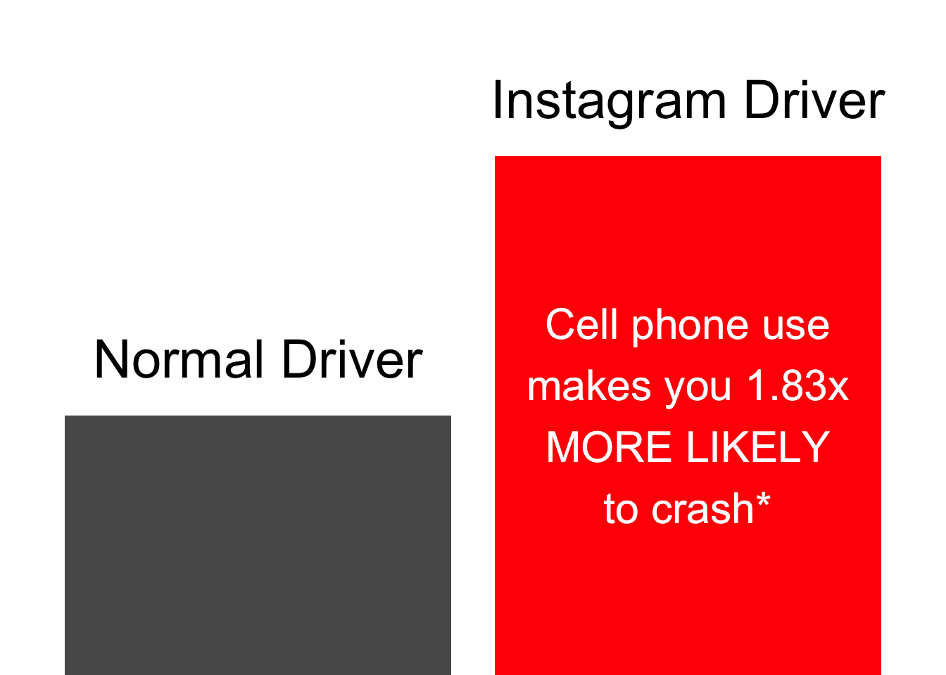
*(based on data from AAA)
The lesson here? For everyone’s sake, please save your Story updates for later!
Conditional Probability in Daily Life
One practical lesson of conditional probability that you can take away is:
If something has failed in the past, pay extra attention to it.
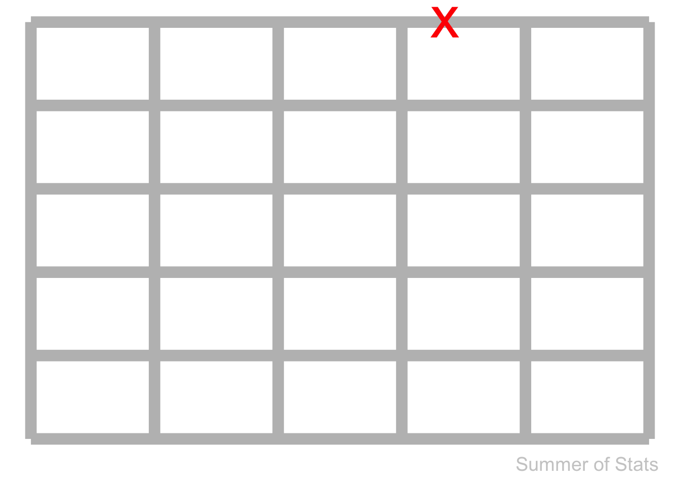
Case-in point: Near my house, there is a small (~50 foot) section of road that has been torn up & re-paved a total of FIVE times. The reason is that the water pipes under this road burst repeatedly.
(side note: I like to joke that this is the “best section of road in Cincinnati”, since it’s been patched and re-paved so many times)
Normally, we wouldn’t expect a single section of pipe would break more than once. Pipe breakages (if they were random) should look like this:
But, our experience looks like this:
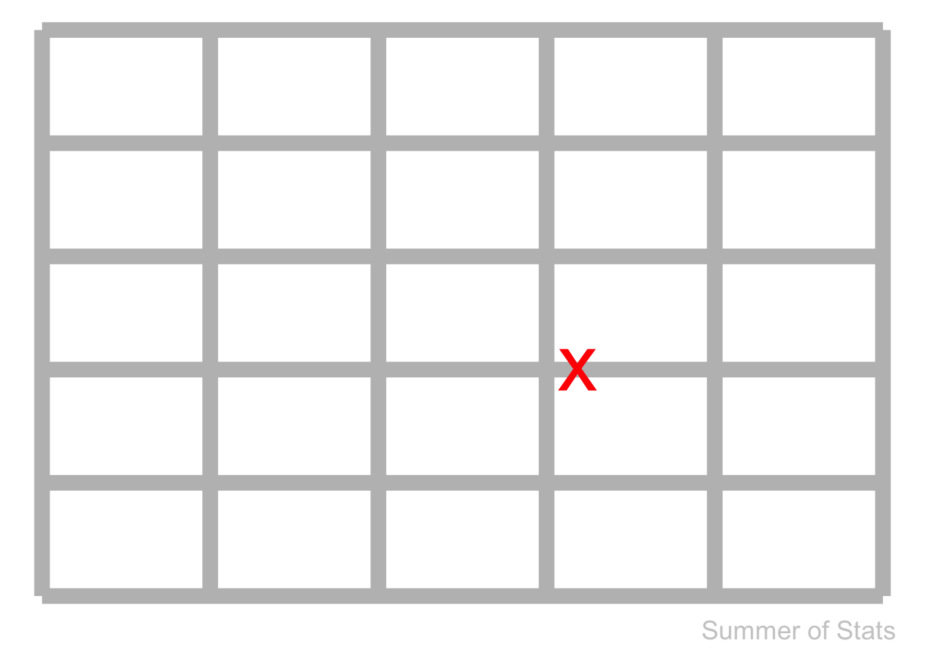
What’s likely happening here is that this problematic section of pipe has something DIFFERENT about it.
Digging deeper…
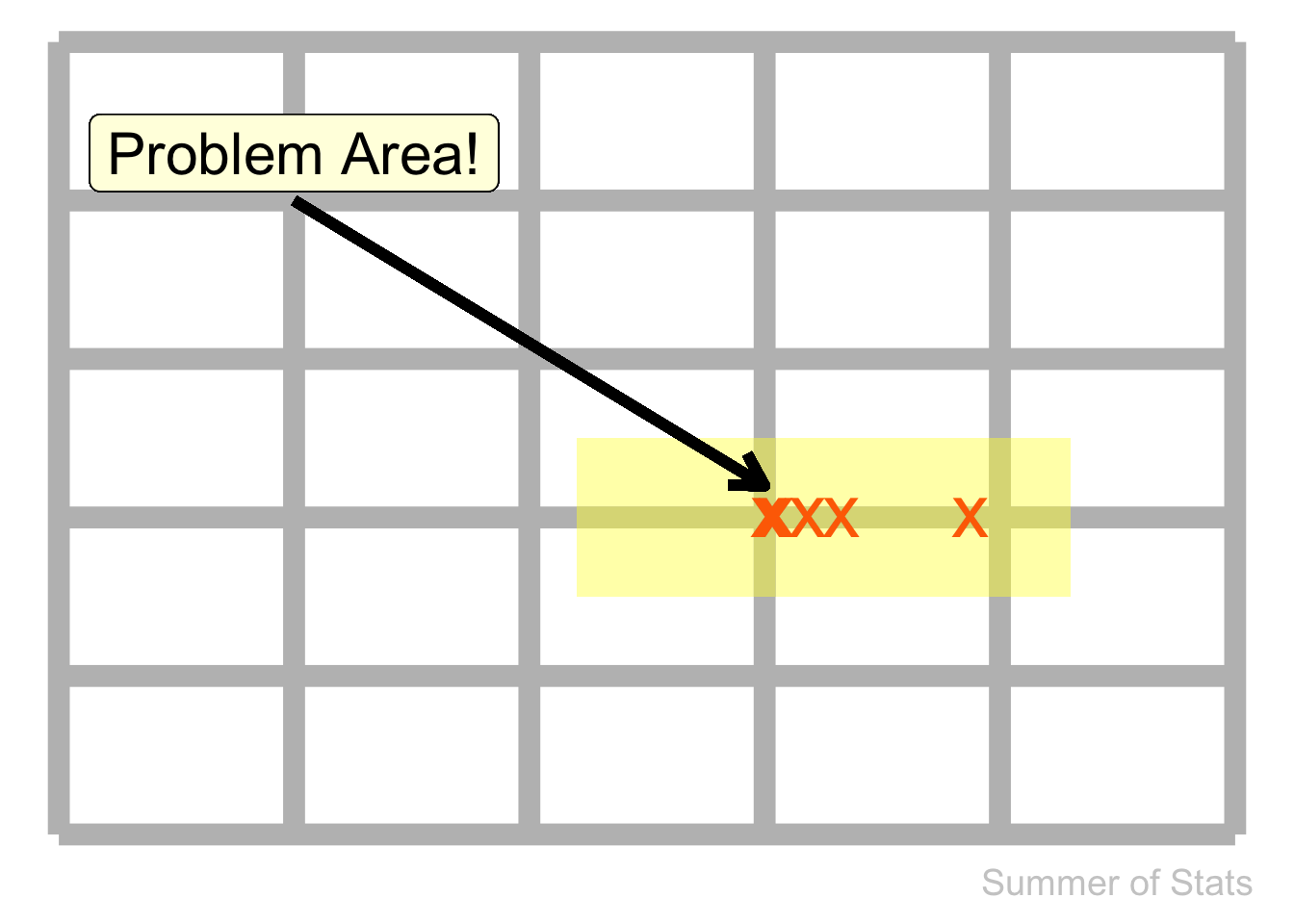
We might decide to dig up this section of pipe (again), to figure out what’s going on. Upon inspection, we find that these pipes are not buried as deeply as they should be, which makes this section of pipe much more likely to burst during a cold snap.
Considering this as a conditional probability problem:
$$ P(burst|normal depth) = 0.0001 $$
$$ P(burst|shallow depth) = 0.1 $$
This framing clearly shows us WHY our shallow section of pipe is bursting much more often — the probability is 1000x higher, given its lack of protection from the elements. We now have our explanation for this odd cluster of failures in 1 spot.
Better yet, we also now have a simple model for predicting future issues - just map out the shallow sections of pipe:
Summing Up
Conditional probability tells us it’s probably a good idea to take an extra look when you’ve experienced a problem.
While it’s not guaranteed you’ll find something odd, there is a chance that SOMETHING could be increasing the likelihood of a failure (such as pipes that aren’t buried deep enough).
If left unaddressed, you may find yourself running into repeated problems, and wondering why you always seem to have such bad luck. In reality, it’s not your luck that is to blame, but conditional probability!
===========================
R code used to generate plots:
- Conditional Risk (Instagram)
library(data.table)
library(ggplot2)

### Accident statistics courtesy of AAA
# A normal driver is expected to have 1 crash every 18 years
# Cell phone use increases relative risk by 1.83
crash_odds <- as.data.table(cbind(
                              c("Overall", "Using Cell"),
                              c(1/18, 1/18 * 1.83)))
setnames(crash_odds, c("DRIVER_TYPE", "P_CRASH"))

### Simple Barplot
ggplot(crash_odds, aes(x=DRIVER_TYPE, y = P_CRASH)) +
  geom_col() +
  geom_col(data = crash_odds[DRIVER_TYPE == "Using Cell"],  aes(x=DRIVER_TYPE, y = P_CRASH), fill = "red") +
  geom_text(label = c("Normal Driver", "Instagram Driver"), vjust = -1, size = 10) +
  geom_text(aes(x = 2, y = 1, label = "Cell phone use\nmakes you 1.83x\nMORE LIKELY\nto crash*"), size = 8, col = "white") +
  theme_void()
- Pipe Bursts
library(data.table)
library(ggplot2)
library(gganimate)
set.seed(060124)

### Create simulated road grid
road_grid <- as.data.table(cbind(rep(1:6, each=6), ## x direction of grid
                                 rep(1:6, 6),  ## y direction of grid
                                 c(rep(0, 20), 1, rep(0,15)), ## shallow depth indicator
                                 c(rep(.0001, 20), 0.1, rep(0.0001, 15))))  ## conditional probability of pipe burst
setnames(road_grid, c("X_DIR", "Y_DIR", "SHALLOW_DEPTH", "COND_PROB"))


##### RANDOM
### Randomly sample 5 observations from our grid
pipe_bursts_rand <- road_grid[X_DIR<5][sample(.N, 5, replace = TRUE)]
pipe_bursts_rand[,ORDER_BY:=.I]

### Plot (Random Selection)
random_plot <- ggplot(road_grid) +
  geom_line(aes(x=X_DIR, y=Y_DIR, group = X_DIR), col = "grey", linewidth = 4) +
  geom_line(aes(x=X_DIR, y=Y_DIR, group = Y_DIR), col = "grey", linewidth = 4) +
  geom_jitter(data = pipe_bursts_rand, aes(x=X_DIR + 0.5, y=Y_DIR, group = ORDER_BY), col = "red", size = 15, width = 0.75, height = 0, shape = 'x') +
        annotate("text", x = 5.5, y = 0.7, label = "Summer of Stats", col="grey80", size = 5) +
  theme_void() +   transition_time(ORDER_BY) +  shadow_mark(colour = 'red', size = 10)

animate(random_plot, duration = 3,end_pause = 50)


##### CONDITIONAL PROBABILITY
### Select 5 observations (conditional probability)
pipe_bursts_cond <- road_grid[sample(.N, 5, replace=TRUE, prob=COND_PROB)]
pipe_bursts_cond[,ORDER_BY:=.I]

### Plot (Conditional Probability)
conditional_plot <- ggplot(road_grid) +
  geom_line(aes(x=X_DIR, y=Y_DIR, group = X_DIR), col = "grey", linewidth = 4) +
  geom_line(aes(x=X_DIR, y=Y_DIR, group = Y_DIR), col = "grey", linewidth = 4) +
  geom_jitter(data = pipe_bursts_cond, aes(x=X_DIR + 0.5, y=Y_DIR, group = ORDER_BY), col = "red", size = 15, width = 0.75, height = 0, shape = 'x') +
        annotate("text", x = 5.5, y = 0.7, label = "Summer of Stats", col="grey80", size = 5) +
  theme_void() + transition_time(ORDER_BY) +  shadow_mark(colour = 'red', size = 10)


animate(conditional_plot, duration = 3,end_pause = 50)

### Plot (Predictions)
prediction_plot <- conditional_plot +
  geom_rect(xmin = 3.2, xmax = 5.3,   ymin = 2.5, ymax = 3.5,   fill = "yellow", alpha = .01) +
  geom_label(aes(x = 2, y = 5.3, label = "Problem Area!"), size = 8, fill = "lightyellow") +
  geom_segment(aes(x = 2, y = 5, xend = 4, yend = 3.2),
                  arrow = arrow(length = unit(0.5, "cm")), linewidth = 2) +
        annotate("text", x = 5.5, y = 0.7, label = "Summer of Stats", col="grey80", size = 5)

prediction_plot